Segmenting Handwritten Bangla Without Deep Learning: An Image Processing Deep Dive

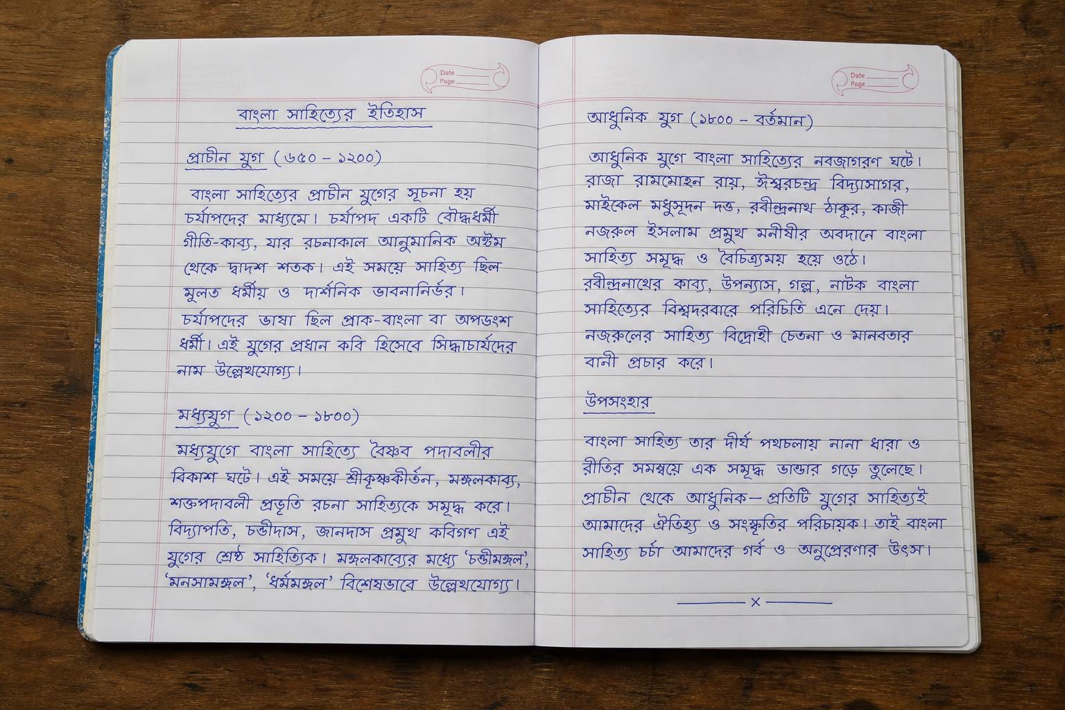
If you take a photo of a handwritten Bangla passage, the challenge addressed by this study arrives before recognizing a single word. A segmentation algorithm must decide which ink strokes belong together and where one word ends and the next begins. Human writers do not always leave the gaps that make those decisions easy.

Closely spaced words can merge into one detected region. Disconnected characters and marks can make a single word look like several.

The authors describe dependable handwritten Bangla OCR as difficult to find. Their research focuses on word segmentation—the stage that slices a page image into individual word regions. Errors here can leave later recognition stages working with incomplete words or several words bundled into one crop.

In their paper, Color Independent Word Segmentation From Transcribed Bangla Passages, researchers Faias Satter, Noor Masrur, and Sk. Md. Masudul Ahsan from Khulna University of Engineering & Technology (KUET) tackle this bottleneck with an adaptive, classical image-processing pipeline. They test smartphone-captured documents with different paper colors, pen types, and shadow interference, extracting word boxes through an iterative contour-counting heuristic. The manuscript was posted to arXiv on October 1, 2026, and identifies itself as the accepted version of a paper published at the 2023 International Conference on Electrical Information and Communication Technology (EICT).

Here is an engineering breakdown of why handwritten Bangla complicates segmentation, how the KUET team designed their pipeline, and what their reported results establish.

The visual geometry of a handwritten script

To understand the segmentation problem, you have to look at the script's physical topography.

Many Bangla characters connect within a word through a horizontal stroke known as the matra. This connection can help keep a word together as an image region, but not every character or mark has a matra, and handwriting does not always preserve a continuous connection.

The paper describes three recurring complications:

1. Matra-less characters and marks create false word breaks. The authors identify signs such as '◌ঃ', '◌ং', and '◌ঁ' as possible sources of splitting errors. Missing connections or gaps within a word can leave its components in separate detected regions.
2. Detached marks complicate word boundaries. Vowel signs such as '◌ু', '◌ূ', 'ি◌', '◌ী', 'ৈ◌', and 'ে◌ৗ' can complicate the separation of neighboring words. The authors describe word components being absorbed into another word, as well as distant marks being excluded from the box around their own word.
3. Variable inter-word spacing. Some writers leave very little space between words and lines. Others write in a scattered style with large gaps between characters inside a word. A setting that joins one writer's disconnected letters can merge another writer's adjacent words.

On top of these script-level dynamics, document capture adds physical messiness. The study includes smartphone images with shadow interference, different image sizes and resolutions, colored inks, and colored paper stocks. These conditions motivate a pipeline that selects its filtering and thresholding settings from the image rather than applying one fixed setting to every page.

Stage 1: Converting phone camera chaos into stable pixels

The KUET team structured their solution as a sequential six-stage pipeline, moving from raw pixels to bounded word regions without executing a separate line-segmentation pass.

The first step converts the incoming image to grayscale. The authors explain that although scanning directly in black and white is faster, some character information may be lost. Grayscale therefore provides the starting point for the subsequent filtering and thresholding stages.

Next comes adaptive noise reduction. Different devices produce images at different resolutions, and different writers produce characters at different scales. The authors use an image-specific metric called Average Contour Size (ACS) to determine filtering settings.

To compute the initial ACS:

• The system runs an initial denoising pass with a Gaussian kernel sized at 21 by 21 pixels. The paper specifies a standard deviation in the vertical direction of 21 and a scaling factor of 7.
• It applies an initial adaptive threshold using a 21 by 21 window.
• It extracts preliminary contours, discarding contours with an area smaller than 50 as salt noise.
• The remaining contour areas provide the ACS used to select later kernel sizes.

Once the system knows the document's ACS, the paper describes the next smoothing stage as Non-local Means Denoising. It also supplies a smoothing-kernel equation using coordinate variables $x$ and $y$, with $\sigma$ defined as the square root of the kernel size. The kernel size itself comes from an empirical ACS lookup table.

Rather than fixing the kernel dimensions, the authors map the calculated ACS to different sizes:

• An ACS below 200 uses a 3 by 3 kernel.
• An ACS from 200 up to, but not including, 300 uses a 5 by 5 kernel.
• The listed sizes increase by 2 across successive 100-unit ACS bands through 1000, reaching 19 by 19 for $900 \le \text{ACS} < 1000$.
• The next entries use 21 by 21 for $1000 \le \text{ACS} < 1200$ and 23 by 23 for $1200 \le \text{ACS} < 1400$.

For extensions beyond the table, the authors describe increasing the kernel size by 2 for every additional 200 units of ACS.

The authors also factor in page background brightness. They report less salt noise for light backgrounds with pixel values between 181 and 255, and more noise as the background gets darker. For background values between 101 and 180, they increase the selected kernel size by 2. For values below 100, they increase it by 4.

These are empirical choices made for the proposed system. They adapt filtering to the estimated contour scale and background brightness, rather than establishing a universal relationship between paper color and the required smoothing strength.

Stage 2: The shadow test and adaptive binarization

Once smoothed, the image must be converted into a binary representation. The pipeline ultimately standardizes this representation as white foreground strokes on a black background.

The authors choose between global thresholding, using Otsu's method, and adaptive thresholding. Their preference is to use Otsu when one threshold is sufficient for the image, while selecting adaptive thresholding for colored backgrounds or shadow interference.

This choice involves a tradeoff. The paper reports that adaptive thresholding can fragment characters because it works within local windows. Parts of a word may then be excluded from its detected contour. Otsu is preferred under suitable conditions because it avoids this fragmentation in the authors' account.

The KUET pipeline performs a shadow-interference check before committing to a binarization method:

$$\frac{\text{Area of largest contour}}{\text{Average Contour Size}} > 100$$

The system applies Otsu thresholding and measures the largest resulting contour. If its area exceeds 100 times the ACS, the pipeline treats the image as having shadow interference. This ratio is the authors' detection heuristic; the paper does not establish that every large contour must be a shadow.

Based on this test and the background pixel intensity, the binarization strategy branches:

• Colored or dark paper, with pixel values below 180: Use adaptive thresholding.
• Light paper, with pixel values at or above 180: Use adaptive thresholding if shadow interference is detected; otherwise, use Otsu thresholding.

The adaptive-thresholding window size comes from the ACS lookup table.

After thresholding, pixel values are inverted where necessary, producing uniform white foreground strokes on a black background. The image then passes through Canny edge detection and a Hough transform to identify co-linear structures used for skew correction.

This skew-correction stage does not divide the page into separate text-line images. Word detection still operates without a preceding line-segmentation pass.

Stage 3: Morphological dilation and the peak-contour stopping point

Now comes the central challenge: grouping disconnected character strokes and detached marks into word entities without bridging the gaps between adjacent words.

The authors rely on mathematical morphology—specifically dilation using a square structuring element with white foreground pixels. Dilation expands foreground regions. It can join components within a word, but further expansion can also connect neighboring words.

Determining the stopping point is the core technical challenge. The authors approach it through a Minimum Area Threshold (MAT) paired with an iterative contour-counting search.

Defining what counts as a word

Before the system can count word candidates, it needs a rule for retaining contours. Connected regions with an area larger than the MAT are counted as candidates and can receive bounding boxes.

Passing the area threshold does not guarantee that a region contains exactly one complete word. It is the pipeline's filtering rule.

Calculating MAT depends on which binarization method was selected earlier:

• After Otsu thresholding: The authors calculate MAT directly from ACS:

$$\text{MAT} = \frac{\text{Average Contour Size}}{1.25}$$

• After adaptive thresholding: The authors account for fragmented contours using a metric called Writing Density (WD):

$$\text{Writing Density} = \frac{\text{Total area of the page}}{\text{Average Contour Size}}$$

The paper interprets a larger WD as less dense writing. Its formula expresses page area relative to average contour area, rather than measuring the gaps between words directly.

The system maps WD to an empirical formula for MAT. The table ranges from $\text{ACS} - \frac{\text{ACS}}{4}$ when $\text{WD} < 1500$ to $\text{ACS} \times 6$ when $\text{WD} \ge 10000$. Intermediate bands use other multiples and fractional adjustments of ACS.

A second table applies further adjustments for combinations of WD and ACS. Its listed rules include subtracting $\frac{\text{ACS}}{8}$ when $\text{WD} > 2000$ and $\text{ACS} > 700$, and adding ACS-based amounts in specified high-WD, high-ACS ranges.

These mappings are empirically selected parts of the method. They are intended to balance retaining word components against accepting small fragments or merging larger regions.

The peak contour search

With MAT defined, the system determines its initial dilation kernel size from ACS. The listed entries begin at 1 by 1 for an ACS below 100 and 3 by 3 for $100 \le \text{ACS} < 1000$. Larger ACS bands receive larger starting kernels, with some differences between the Otsu and adaptive-thresholding branches.

For example, the table assigns a 9 by 9 starting kernel after Otsu and an 11 by 11 kernel after adaptive thresholding when $2000 \le \text{ACS} < 2200$. The listed adaptive-thresholding entries reach 13 by 13 for $2400 \le \text{ACS} < 2600$; this is not presented as a maximum for all images.

The algorithm dilates the binary image with the starting kernel for one iteration and counts contours whose areas exceed MAT. It then tests further settings, increasing either the iteration count or the kernel size, and recounts the retained contours.

The contour-counting heuristic rests on two effects:

• Disconnected components can join into regions large enough to exceed MAT, increasing the number of retained word candidates.
• Neighboring word regions can merge during further dilation, reducing the contour count.

The authors describe searching for the maximum contour count and stopping before further dilation causes words to collide. This is a heuristic for selecting a dilation setting. It does not guarantee that every word is complete or that every neighboring pair remains separate at the chosen point.

In one example documented in the paper's Figure 4, an image with an ACS of 641 starts with a 3 by 3 dilation kernel. Using that kernel for 3 iterations produces 33 detected words at the illustrated optimal setting. A 10 by 10 kernel applied for 2 iterations produces only 23.

Finally, rectangular bounding boxes are fitted around the retained word contours at the selected setting.

Benchmarks: Testing on three distinct datasets

To evaluate their approach, the KUET team tested the pipeline across three document collections: a bespoke dataset created for the project, CMATERdb1.1.1, and the collection the paper calls the Bangla Writing dataset.

1. The custom 80-document dataset

To evaluate varied capture conditions, the authors built an 80-document dataset spanning different handwriting styles, written on white, red, blue, green, and black papers. They used gel, ballpoint, and glittering pens in different colors, including black, red, green, and blue.

They also introduced shadow interference and used different capture devices so that the images varied in size and resolution.

The paper reports:

• Ground truth words: 7,374
• Bounding boxes generated: 7,278
• Correctly segmented words: 6,681
• Segmentation errors: 527 words, classified as under-segmented, over-segmented, or defect-segmented
• Undetected words: 166
• Recall: 90.60%
• Precision: 91.80%
• F1-score: 91.20%

These results demonstrate the method on the authors' color-varied, shadow-containing collection. They do not establish reliable segmentation for every possible combination of paper, ink, handwriting, and lighting.

2. CMATERdb1.1.1 benchmark

The authors ran the pipeline across 100 documents from CMATERdb1.1.1, generating 15,587 bounding boxes across 15,730 words:

• Correctly segmented: 13,552 words
• Segmentation errors: 2,048 words
• Undetected: 130 words
• Recall: 86.15%
• Precision: 86.94%
• F1-score: 86.54%

For comparison, the paper reports that Sarkar et al. (2011) obtained a word-segmentation success rate of 86.01%: 13,530 correctly segmented words out of 15,730, with 2,200 words either under-segmented or over-segmented.

The input distinction matters. According to the KUET paper, Sarkar et al. used document images already segmented into text lines, whereas the proposed method does not require that preprocessing stage.

The proposed method's reported recall is slightly higher than the earlier success rate. The differing input conditions, however, mean this is not a controlled demonstration of an overall performance advantage.

3. Bangla Writing dataset

The system was also evaluated on 100 documents from the Bangla Writing dataset:

• Total words present: 7,400
• Bounding boxes generated: 7,191
• Correctly segmented: 6,380 words
• Segmentation errors: 987 words
• Undetected: 33 words
• Recall: 86.22%
• Precision: 88.72%
• F1-score: 87.45%

The paper reports that Das et al. (2023) worked on a portion of this dataset using horizontal projection profiles, seam carving, and contour tracing. Their reported results were 88.39% line-segmentation accuracy, 95.65% word-segmentation accuracy, and 84.55% average accuracy.

The KUET comparison table places that 84.55% average accuracy beside the proposed method's recall, precision, and F1-score. These are different measures, and the evaluations use different dataset portions. The 87.45% F1-score therefore should not be read as a directly comparable improvement over the earlier average accuracy.

How the pipeline breaks down: four error modes

Because the algorithm uses image geometry rather than recognizing the text, its reported failures follow geometric edge cases. The authors classify them into four error types.

The labels below follow the paper's terminology: it calls word splitting under-segmentation and word merging over-segmentation.

1. Under-segmentation error (word splitting): A single word is split into two or more bounding boxes. The authors associate this with missing matra connections, unusually wide gaps between internal characters, and matra-less signs such as '◌ঃ', '◌ং', and '◌ঁ'.
2. Over-segmentation error (word merging): A single bounding box contains two or more words. Dense handwriting with insufficient gaps between words or lines increases the likelihood of this error.
3. Defect-segmentation error (excluded marks): A bounding box surrounds a word but leaves part of it outside. The paper gives examples involving vowel signs and other marks, including '◌া', 'ি◌', '◌ঁ', '◌ৃ', and '◌ী', especially when they are written far from the main word body.
4. Overlooking error (missed words): A word is omitted from the output. The authors identify words with small areas as vulnerable when the minimum area threshold is increased.

These errors create competing tuning pressures. A smaller starting dilation kernel or smaller MAT can help with densely written pages, but the authors report that such choices can increase splitting errors in scattered handwriting. A smaller dilation kernel can also leave distant marks outside a word's box.

Punctuation presents another complication. The paper reports that marks such as the Bangla sentence-ending daari ('।') and commas can be detected with neighboring words. In some handwriting styles, they instead receive individual bounding boxes.

Finally, the background surrounding the paper can generate false detections when its pixel values resemble those of the characters. The authors propose cropping the image to remove that background.

Why it matters for document parsing and OCR systems

The KUET paper offers a detailed example of word segmentation built from classical image-processing operations. Its contribution is a method for producing word regions, evaluated through segmentation counts and metrics.

It does not evaluate recognition of the words inside those regions. The distinction matters when interpreting the results: a correctly segmented crop is an input to later OCR stages, not evidence that its text has been correctly transcribed.

Eliminating the line segmentation dependency

A segmentation workflow can proceed through a hierarchy such as:

$$\text{Page} \longrightarrow \text{Text Lines} \longrightarrow \text{Words} \longrightarrow \text{Characters}$$

In such a workflow, errors in line segmentation can affect subsequent word extraction. The paper's discussion of related work identifies difficulties when handwritten lines overlap or when their extents differ substantially.

The proposed method extracts word regions without first dividing the document into separate lines. The authors argue that this avoids making word extraction depend on a successful line-segmentation stage.

This does not eliminate errors caused by crowded words and lines. Those conditions still appear in the paper's failure analysis. The benefit is the removal of that separate preprocessing dependency, rather than a guarantee that segmentation errors remain confined to one word pair.

Classical processing, without a runtime benchmark

The described pipeline uses grayscale conversion, denoising, thresholding, Canny edge detection, a Hough transform, and morphological dilation. No deep-learning model is part of the proposed segmentation method.

That makes the paper useful as a worked example of a classical approach. It does not, however, establish a particular execution speed or deployment cost.

The study reports segmentation results but provides no runtime, memory, energy-use, or on-device execution benchmark. Smartphone-captured images describe the input source; they do not demonstrate that the processing ran on a smartphone.

Claims about millisecond execution, low-end phone performance, battery consumption, or advantages over neural systems would therefore go beyond the reported evidence.

The limits of empirical lookup tables

The paper also exposes the tuning demands of this approach.

Its mapping tables link ACS and WD to smoothing kernels, area thresholds, and starting dilation kernels. These tables use discrete intervals: an ACS of 299 selects a 5 by 5 smoothing kernel, while an ACS of 301 selects a 7 by 7 kernel.

That means a small change across a table boundary can change a processing parameter. The paper does not measure sensitivity at those boundaries or establish that the mappings transfer reliably to every new capture condition.

The authors' error analysis shows why tuning is difficult. Increasing dilation can join disconnected parts of a word while also merging adjacent words. Raising the area threshold can exclude smaller words. Different handwriting styles pull these settings in different directions.

The proposed improvements stay close to those observed failures. The authors suggest nested processing of bounding boxes containing multiple words and more precise adjustment of adaptive-thresholding and dilation filter sizes. For words with almost no separating gaps, they also propose a machine-learning model trained on dictionary words.

These are future directions, not evaluated extensions of the reported pipeline.

Satter, Masrur, and Ahsan show how an adaptive classical pipeline can segment handwritten Bangla across several datasets, including their collection of colored-paper and shadow-affected photographs. Its contour-counting search and detailed failure analysis provide a concrete contribution to word segmentation—and a starting point for the later recognition stages needed to turn those boxes into editable text.